Some of the following problems appeared in the exercises in the coursera course Image Processing (by Northwestern University). The following descriptions of the problems are taken directly from the assignment’s description.
1. Some Information and Coding Theory
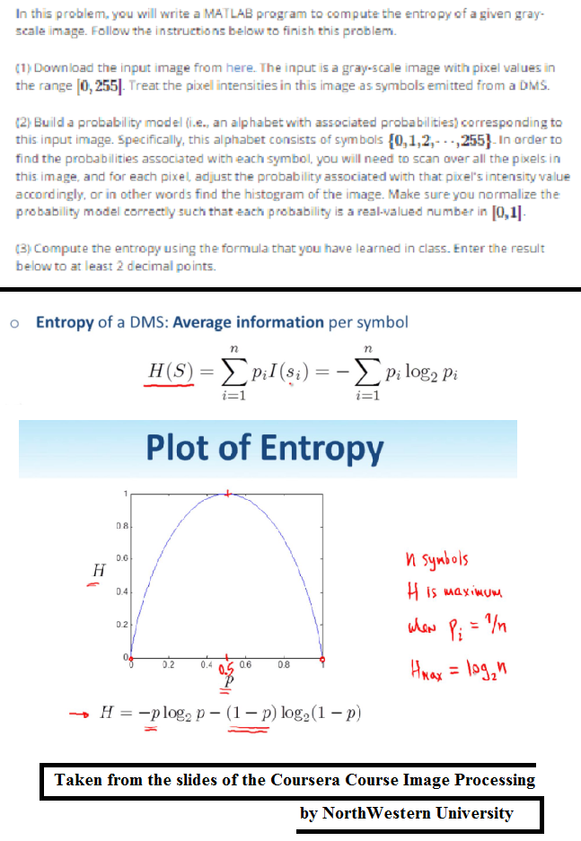
Computing the Entropy of an Image
The next figure shows the problem statement. Although it was originally implemented in MATLAB, in this article a python implementation is going to be described.
Histogram Equalization and Entropy
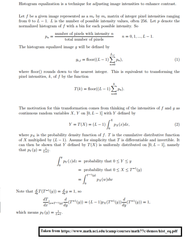
Histogram equalization is a well-known image transformation technique to imrpove the contrast of an image. The following figure shows the theory for the technique: each pixel is transformed by the CDF of the image and as can be shown, the output image is expected to follow an uniform distribution (and thereby with the highest entropy) over the pixel intensities (as proved), considering the continuous pixel density. But since the pixel values are discrete (integers), the result obtained is going to be near-uniform.
The following figures show a few images and the corresponding equalized images and how the PMF and CDF changes.
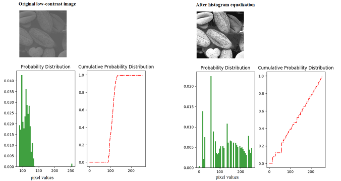
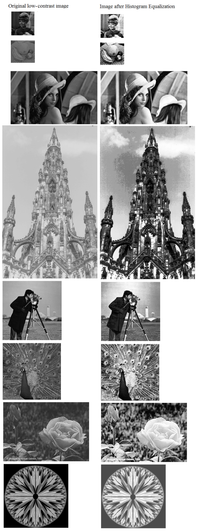
Image Data Compression with Huffman and Lempel Ziv (LZ78) Coding
Now let’s implement the following couple of compression techniques:
- Huffman Coding
- Lempel-Ziv Coding (LZ78)
and compress a few images and their histogram equalized versions and compare the entropies.
The following figure shows the theory and the algorithms to be implemented for these two source coding techniques:
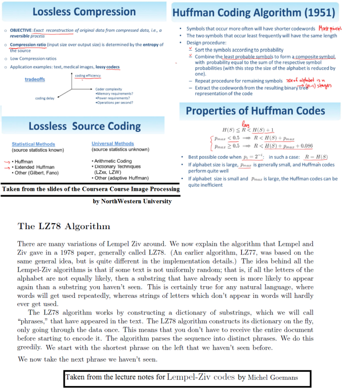
Let’s now implement the Huffman Coding algorithm to compress the data for a few gray-scale images.
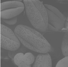
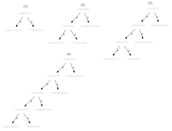
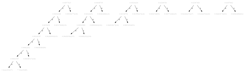
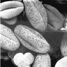
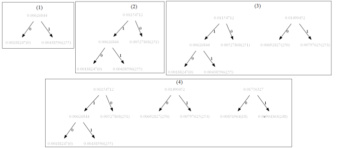
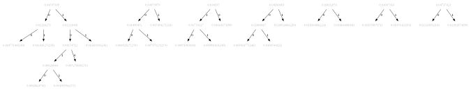
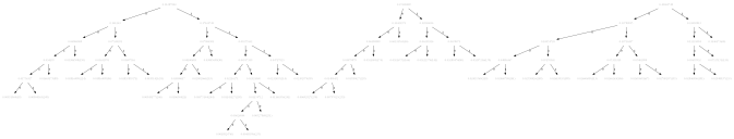
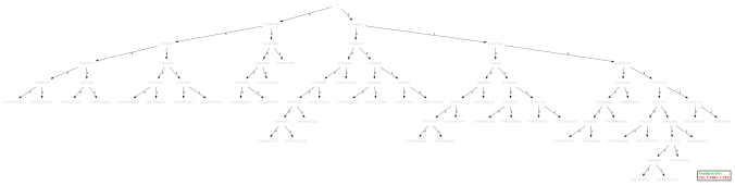
The following figures show how the tree is getting constructed with the Huffman Coding algorithm (the starting, final and a few intermediate steps) for the following low-contrast image beans. Here we have alphabets from the set {0,1,…,255}, only the pixels present in the image are used. It takes 44 steps to construct the tree.


The following table shows the Huffman Codes for different pixel values for the above low-contrast image beans.
| index | pixel | code |
|---|---|---|
| 15 | 108 | 0 |
| 3 | 115 | 1 |
| 20 | 109 | 10 |
| 1 | 112 | 11 |
| 32 | 107 | 100 |
| 44 | 110 | 101 |
| 18 | 96 | 110 |
| 11 | 95 | 111 |
| 21 | 120 | 1000 |
| 35 | 91 | 1001 |
| 6 | 116 | 1010 |
| 24 | 123 | 1011 |
| 2 | 98 | 1100 |
| 13 | 100 | 1101 |
| 17 | 94 | 1111 |
| 12 | 119 | 10000 |
| 4 | 114 | 10001 |
| 42 | 103 | 10011 |
| 16 | 106 | 10100 |
| 37 | 132 | 10101 |
| 41 | 130 | 10111 |
| 5 | 117 | 11000 |
| 26 | 125 | 11010 |
| 40 | 99 | 11011 |
| 38 | 118 | 11100 |
| 0 | 113 | 11101 |
| 22 | 121 | 11111 |
| 39 | 131 | 101011 |
| 27 | 127 | 101111 |
| 31 | 102 | 110011 |
| 25 | 124 | 110101 |
| 23 | 122 | 110111 |
| 33 | 104 | 111011 |
| 34 | 105 | 111111 |
| 29 | 129 | 1001111 |
| 30 | 93 | 1010101 |
| 7 | 137 | 1010111 |
| 14 | 255 | 1101011 |
| 28 | 128 | 1101111 |
| 36 | 133 | 11010111 |
| 10 | 134 | 11101011 |
| 9 | 135 | 101010111 |
| 43 | 90 | 1001010111 |
| 8 | 136 | 10001010111 |
| 19 | 89 | 100001010111 |
- First construct the tree for the equalized image.
- Use the tree to encode the image data and then compare the compression ratio with the one obtained using the same algorithm with the low-contrast image.
- Find if the histogram equalization increases / reduces the compression ratio or equivalently the entropy of the image.
The following figures show how the tree is getting constructed with the Huffman Coding algorithm (the starting, final and a few intermediate steps) for the image beans. Here we have alphabets from the set {0,1,…,255}, only the pixels present in the image are used. It takes 40 steps to construct the tree, also as can be seen from the following figures the tree constructed is structurally different from the one constructed on the low-contract version of the same image.


The following table shows the Huffman Codes for different pixel values for the above high-contrast image beans.
| index | pixel | code |
|---|---|---|
| 13 | 119 | 0 |
| 11 | 250 | 1 |
| 5 | 133 | 10 |
| 0 | 150 | 11 |
| 8 | 113 | 100 |
| 32 | 166 | 101 |
| 36 | 60 | 110 |
| 40 | 30 | 111 |
| 25 | 208 | 1000 |
| 38 | 16 | 1001 |
| 21 | 181 | 1010 |
| 33 | 224 | 1011 |
| 9 | 67 | 1100 |
| 37 | 80 | 1101 |
| 27 | 244 | 1111 |
| 23 | 201 | 10000 |
| 17 | 174 | 10001 |
| 6 | 89 | 10011 |
| 34 | 106 | 10100 |
| 24 | 141 | 10101 |
| 28 | 246 | 10111 |
| 22 | 188 | 11000 |
| 10 | 235 | 11010 |
| 30 | 71 | 11011 |
| 2 | 195 | 11100 |
| 3 | 158 | 11101 |
| 1 | 214 | 11111 |
| 31 | 228 | 100001 |
| 15 | 84 | 101011 |
| 12 | 251 | 101111 |
| 39 | 18 | 110011 |
| 4 | 219 | 110111 |
| 14 | 93 | 111011 |
| 26 | 99 | 111111 |
| 19 | 253 | 1000001 |
| 7 | 238 | 1001111 |
| 18 | 21 | 1010111 |
| 29 | 241 | 1101111 |
| 35 | 248 | 1110011 |
| 20 | 0 | 10101111 |
| 16 | 255 | 110101111 |
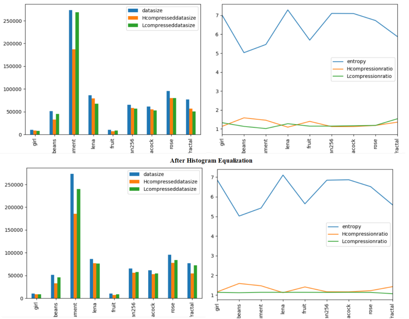
The following figure shows the compression ratio for different images using Huffman and LZ78 codes, both on the low-contrast and high contrast images (obtained using histogram equalization). The following observations can be drawn from the comparative results shown in the following figures (here H represents Huffman and L represents LZ78):
- The entropy of an image stays almost the same after histogram equalization
- The compression ratio with Huffman / LZ78 also stays almost the same with an image with / without histogram equalization.
- The Huffman codes achieves higher compression in some cases than LZ78.
The following shows the first few symbol/code pairs for the dictionary obtained with LZ78 algorithm, with the alphabet set as {0,1,..,255} for the low-contrast beans image (there are around 18k codes in the dictionary for this image):
| index | symbol (pixels) | code |
| 7081 | 0 | 0 |
|---|---|---|
| 10325 | 1 | 1 |
| 1144 | 2 | 10 |
| 7689 | 4 | 100 |
| 8286 | 8 | 1000 |
| 7401 | 16 | 10000 |
| 8695 | 32 | 100000 |
| 10664 | 64 | 1000000 |
| 5926 | 128 | 10000000 |
| 7047 | 128,128 | 1000000010000000 |
| 1608 | 128,128,128 | 100000001000000010000000 |
| 12399 | 128,128,128,128 | 10000000100000001000000010000000 |
| 3224 | 128,128,128,128,128 | 1000000010000000100000001000000010000000 |
| 3225 | 128,128,128,128,129 | 1000000010000000100000001000000010000001 |
| 3231 | 128,128,128,128,127 | 100000001000000010000000100000001111111 |
| 12398 | 128,128,128,129 | 10000000100000001000000010000001 |
| 12401 | 128,128,128,123 | 1000000010000000100000001111011 |
| 12404 | 128,128,128,125 | 1000000010000000100000001111101 |
| 12403 | 128,128,128,127 | 1000000010000000100000001111111 |
| 1609 | 128,128,129 | 100000001000000010000001 |
| 8780 | 128,128,129,128 | 10000000100000001000000110000000 |
| 7620 | 128,128,130 | 100000001000000010000010 |
| 2960 | 128,128,130,125 | 1000000010000000100000101111101 |
| 2961 | 128,128,130,127 | 1000000010000000100000101111111 |
| 8063 | 128,128,118 | 10000000100000001110110 |
| 1605 | 128,128,121 | 10000000100000001111001 |
| 6678 | 128,128,121,123 | 100000001000000011110011111011 |
| 1606 | 128,128,122 | 10000000100000001111010 |
| 1601 | 128,128,124 | 10000000100000001111100 |
| 1602 | 128,128,125 | 10000000100000001111101 |
| … | … | … |
| 4680 | 127,127,129 | 1111111111111110000001 |
| 2655 | 127,127,130 | 1111111111111110000010 |
| 1254 | 127,127,130,128 | 111111111111111000001010000000 |
| 7277 | 127,127,130,129 | 111111111111111000001010000001 |
| 9087 | 127,127,120 | 111111111111111111000 |
| 9088 | 127,127,122 | 111111111111111111010 |
| 595 | 127,127,122,121 | 1111111111111111110101111001 |
| 9089 | 127,127,123 | 111111111111111111011 |
| 9090 | 127,127,124 | 111111111111111111100 |
| 507 | 127,127,124,120 | 1111111111111111111001111000 |
| 508 | 127,127,124,125 | 1111111111111111111001111101 |
| 9091 | 127,127,125 | 111111111111111111101 |
| 9293 | 127,127,125,129 | 11111111111111111110110000001 |
| 2838 | 127,127,125,132 | 11111111111111111110110000100 |
| 1873 | 127,127,125,116 | 1111111111111111111011110100 |
| 9285 | 127,127,125,120 | 1111111111111111111011111000 |
| 9284 | 127,127,125,125 | 1111111111111111111011111101 |
| 10394 | 127,127,125,125,131 | 111111111111111111101111110110000011 |
| 4357 | 127,127,125,125,123 | 11111111111111111110111111011111011 |
| 4358 | 127,127,125,125,125 | 11111111111111111110111111011111101 |
| 6615 | 127,127,125,125,125,124 | 111111111111111111101111110111111011111100 |
| 9283 | 127,127,125,127 | 1111111111111111111011111111 |
| 9092 | 127,127,127 | 111111111111111111111 |
| 1003 | 127,127,127,129 | 11111111111111111111110000001 |
| 7031 | 127,127,127,130 | 11111111111111111111110000010 |
| 1008 | 127,127,127,121 | 1111111111111111111111111001 |
| 1009 | 127,127,127,122 | 1111111111111111111111111010 |
| 1005 | 127,127,127,125 | 1111111111111111111111111101 |
| 2536 | 127,127,127,125,125 | 11111111111111111111111111011111101 |
| 5859 | 127,127,127,127 | 1111111111111111111111111111 |
12454 rows × 2 columns
The next table shows the dictionary obtained for the high-contrast beans image using LZ78 algorithm:
2. Spatial Domain Watermarking: Embedding images into images
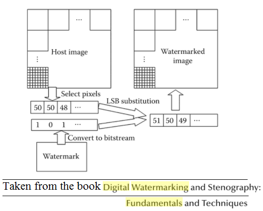
The following figure describes the basics of spatial domain digital watermarking:
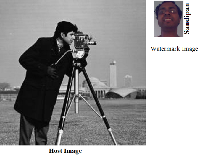
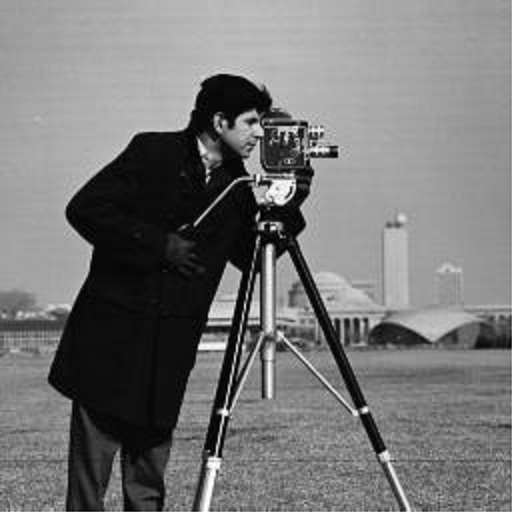
The next figures show the watermark image and the grayscale host image to be used for embedding the watermark image inside the host image.
 The next animations show the embedding of the most significant bit for each pixel of the watermark image inside the gray-scale host image at the upper-left corner at the bits 0,1,…,7 respectively, for each pixel in the host image. As expected, when embedded into a higher significant bit of the host image, the watermark becomes more prominent than when embedded into a lower significant bit.
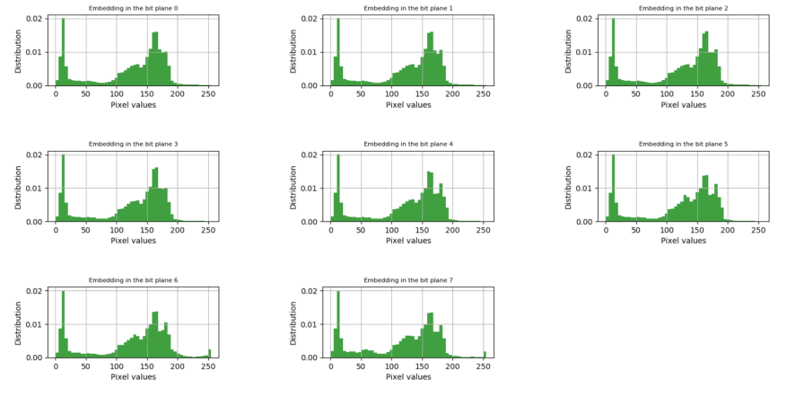
The next figure shows how the distribution of the pixel intensities change when embedding into different bits.

Pingback: Sandipan Dey: Some Image Processing, Information and Coding Theory with Python | Adrian Tudor Web Designer and Programmer