Some Deep Learning with Python, TensorFlow and Keras

 

The following problems are taken from a few assignments from the coursera courses Introduction to Deep Learning (by Higher School of Economics) and Neural Networks and Deep Learning (by Prof Andrew Ng, deeplearning.ai). The problem descriptions are taken straightaway from the assignments.

 

1. Linear models, Optimization

In this assignment a linear classifier will be implemented and it will be trained using stochastic gradient descent with numpy.

Two-dimensional classification

To make things more intuitive, let’s solve a 2D classification problem with synthetic data.

Features

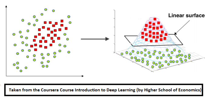
As we  can notice the data above isn’t linearly separable. Hence we should add features (or use non-linear model). Note that decision line between two classes have form of circle, since that we can add quadratic features to make the problem linearly separable. The idea under this displayed on image below:

Here are some test results for the implemented expand function, that is used for adding quadratic features:

# simple test on random numbers

dummy_X = np.array([
        [0,0],
        [1,0],
        [2.61,-1.28],
        [-0.59,2.1]
    ])

# call expand function
dummy_expanded = expand(dummy_X)

# what it should have returned:   x0       x1       x0^2     x1^2     x0*x1    1
dummy_expanded_ans = np.array([[ 0.    ,  0.    ,  0.    ,  0.    ,  0.    ,  1.    ],
                               [ 1.    ,  0.    ,  1.    ,  0.    ,  0.    ,  1.    ],
                               [ 2.61  , -1.28  ,  6.8121,  1.6384, -3.3408,  1.    ],
                               [-0.59  ,  2.1   ,  0.3481,  4.41  , -1.239 ,  1.    ]])

 

Logistic regression

To classify objects we will obtain probability of object belongs to class ‘1’. To predict probability we will use output of linear model and logistic function:

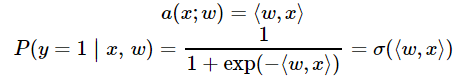
def probability(X, w):
    """
    Given input features and weights
    return predicted probabilities of y==1 given x, P(y=1|x), see description above
        
    :param X: feature matrix X of shape [n_samples,6] (expanded)
    :param w: weight vector w of shape [6] for each of the expanded features
    :returns: an array of predicted probabilities in [0,1] interval.
    """

    return 1. / (1 + np.exp(-np.dot(X, w)))

In logistic regression the optimal parameters w are found by cross-entropy minimization:

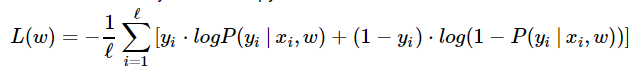
def compute_loss(X, y, w):
    """
    Given feature matrix X [n_samples,6], target vector [n_samples] of 1/0,
    and weight vector w [6], compute scalar loss function using formula above.
    """
    return -np.mean(y*np.log(probability(X, w)) + (1-y)*np.log(1-probability(X, w)))

Since we train our model with gradient descent, we should compute gradients. To be specific, we need the following derivative of loss function over each weight:

Here is the derivation (can be found here too):

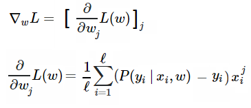
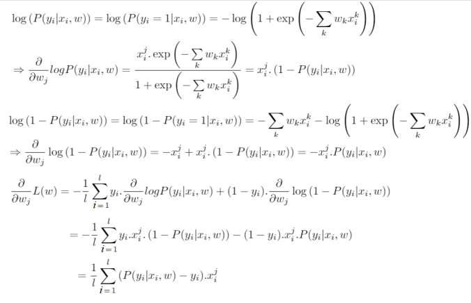
def compute_grad(X, y, w):
    """
    Given feature matrix X [n_samples,6], target vector [n_samples] of 1/0,
    and weight vector w [6], compute vector [6] of derivatives of L over each weights.
    """
    
    return np.dot((probability(X, w) - y), X) / X.shape[0]

Training

In this section we’ll use the functions we wrote to train our classifier using stochastic gradient descent. We shall try to change hyper-parameters like batch size, learning rate and so on to find the best one.

Mini-batch SGD

Stochastic gradient descent just takes a random example on each iteration, calculates a gradient of the loss on it and makes a step:

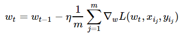
w = np.array([0, 0, 0, 0, 0, 1]) # initialize

eta = 0.05 # learning rate
n_iter = 100
batch_size = 4
loss = np.zeros(n_iter)

for i in range(n_iter):
    ind = np.random.choice(X_expanded.shape[0], batch_size)
    loss[i] = compute_loss(X_expanded, y, w)
    dw = compute_grad(X_expanded[ind, :], y[ind], w)
    w = w - eta*dw

The following animation shows how the decision surface and the cross-entropy loss function changes with different batches with SGD where batch-size=4.

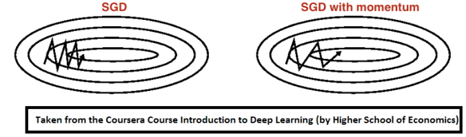
SGD with momentum

Momentum is a method that helps accelerate SGD in the relevant direction and dampens oscillations as can be seen in image below. It does this by adding a fraction α of the update vector of the past time step to the current update vector.

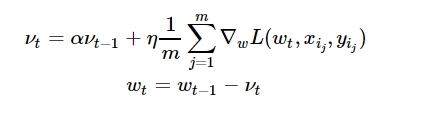
eta = 0.05 # learning rate
alpha = 0.9 # momentum
nu = np.zeros_like(w)
n_iter = 100
batch_size = 4
loss = np.zeros(n_iter)

for i in range(n_iter):
    ind = np.random.choice(X_expanded.shape[0], batch_size)
    loss[i] = compute_loss(X_expanded, y, w)
    dw = compute_grad(X_expanded[ind, :], y[ind], w)
    nu = alpha*nu + eta*dw
    w = w - nu

The following animation shows how the decision surface and the cross-entropy loss function changes with different batches with SGD + momentum  where batch-size=4. As can be seen, the loss function drops much faster, leading to a faster convergence.

RMSprop

We also need to implement RMSPROP algorithm, which use squared gradients to adjust learning rate as follows:

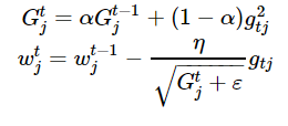
eta = 0.05 # learning rate
alpha = 0.9 # momentum
G = np.zeros_like(w)
eps = 1e-8
n_iter = 100
batch_size = 4
loss = np.zeros(n_iter)

for i in range(n_iter):
    ind = np.random.choice(X_expanded.shape[0], batch_size)
    loss[i] = compute_loss(X_expanded, y, w)
     dw = compute_grad(X_expanded[ind, :], y[ind], w)
     G = alpha*G + (1-alpha)*dw**2
     w = w - eta*dw / np.sqrt(G + eps)

The following animation shows how the decision surface and the cross-entropy loss function changes with different batches with SGD + RMSProp where batch-size=4. As can be seen again, the loss function drops much faster, leading to a faster convergence.

2. Planar data classification with a neural network with one hidden layer, an implementation from scratch

In this assignment a neural net with a single hidden layer will be trained from scratch. We shall see a big difference between this model and the one implemented using logistic regression.

We shall learn how to:

• Implement a 2-class classification neural network with a single hidden layer
• Use units with a non-linear activation function, such as tanh
• Compute the cross entropy loss
• Implement forward and backward propagation

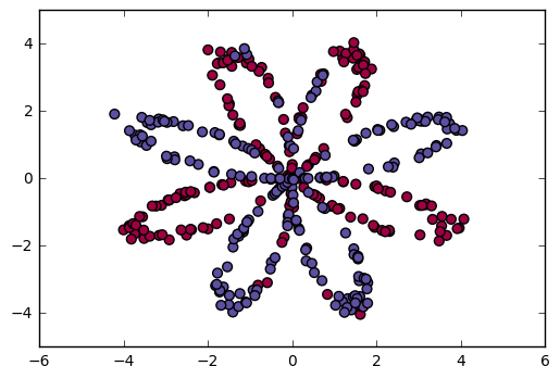
Dataset

The following figure visualizes a “flower” 2-class dataset that we shall work on, the colors indicates the class labels.  We have m = 400 training examples.

Simple Logistic Regression

Before building a full neural network, lets first see how logistic regression performs on this problem. We can use sklearn’s built-in functions to do that, by running the code below to train a logistic regression classifier on the dataset.

# Train the logistic regression classifier
clf = sklearn.linear_model.LogisticRegressionCV();
clf.fit(X.T, Y.T);

We can now plot the decision boundary of the model and accuracy with the following code.

# Plot the decision boundary for logistic regression
plot_decision_boundary(lambda x: clf.predict(x), X, Y)
plt.title("Logistic Regression")

# Print accuracy
LR_predictions = clf.predict(X.T)
print ('Accuracy of logistic regression: %d ' % float((np.dot(Y,LR_predictions) + np.dot(1-Y,1-LR_predictions))/float(Y.size)*100) +
       '% ' + "(percentage of correctly labelled datapoints)")

Accuracy of logistic regression: 47 % (percentage of correctly labelled datapoints)

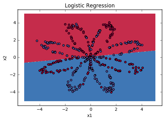
Accuracy

47%

Interpretation: The dataset is not linearly separable, so logistic regression doesn’t perform well. Hopefully a neural network will do better. Let’s try this now!

 

Neural Network model

Logistic regression did not work well on the “flower dataset”. We are going to train a Neural Network with a single hidden layer, by implementing the network with python numpy from scratch.

Here is our model:

The general methodology to build a Neural Network is to:

1. Define the neural network structure ( # of input units,  # of hidden units, etc). 
2. Initialize the model's parameters
3. Loop:
    - Implement forward propagation
    - Compute loss
    - Implement backward propagation to get the gradients
    - Update parameters (gradient descent)

Defining the neural network structure

Define three variables and the function layer_sizes:

- n_x: the size of the input layer
- n_h: the size of the hidden layer (set this to 4) 
- n_y: the size of the output layer

def layer_sizes(X, Y):
    """
    Arguments:
    X -- input dataset of shape (input size, number of examples)
    Y -- labels of shape (output size, number of examples)
    
    Returns:
    n_x -- the size of the input layer
    n_h -- the size of the hidden layer
    n_y -- the size of the output layer
    """

Initialize the model’s parameters

Implement the function initialize_parameters().

Instructions:

• Make sure the parameters’ sizes are right. Refer to the neural network figure above if needed.
• We will initialize the weights matrices with random values.
  • Use: np.random.randn(a,b) * 0.01 to randomly initialize a matrix of shape (a,b).
• We will initialize the bias vectors as zeros.
  • Use: np.zeros((a,b)) to initialize a matrix of shape (a,b) with zeros.

def initialize_parameters(n_x, n_h, n_y):
    """
    Argument:
    n_x -- size of the input layer
    n_h -- size of the hidden layer
    n_y -- size of the output layer
    
    Returns:
    params -- python dictionary containing the parameters:
                    W1 -- weight matrix of shape (n_h, n_x)
                    b1 -- bias vector of shape (n_h, 1)
                    W2 -- weight matrix of shape (n_y, n_h)
                    b2 -- bias vector of shape (n_y, 1)
    """

The Loop

Implement forward_propagation().

Instructions:

• Look above at the mathematical representation of the classifier.
• We can use the function sigmoid().
• We can use the function np.tanh(). It is part of the numpy library.
• The steps we have to implement are:
  1. Retrieve each parameter from the dictionary “parameters” (which is the output of initialize_parameters()) by using parameters[".."].
  2. Implement Forward Propagation. Compute Z[1],A[1],Z[2]Z[1],A[1],Z[2] and A[2]A[2] (the vector of all the predictions on all the examples in the training set).
• Values needed in the backpropagation are stored in “cache“. The cache will be given as an input to the backpropagation function.

def forward_propagation(X, parameters):
    """
    Argument:
    X -- input data of size (n_x, m)
    parameters -- python dictionary containing the parameters (output of initialization function)
    
    Returns:
    A2 -- The sigmoid output of the second activation
    cache -- a dictionary containing "Z1", "A1", "Z2" and "A2"
    """

Implement compute_cost() to compute the value of the cost J.  There are many ways to implement the cross-entropy loss.

def compute_cost(A2, Y, parameters):
    """
    Computes the cross-entropy cost given in equation (13)
    
    Arguments:
    A2 -- The sigmoid output of the second activation, of shape (1, number of examples)
    Y -- "true" labels vector of shape (1, number of examples)
    parameters -- python dictionary containing the parameters W1, b1, W2 and b2
    
    Returns:
    cost -- cross-entropy cost given equation (13)
    """    

Using the cache computed during forward propagation, we can now implement backward propagation.

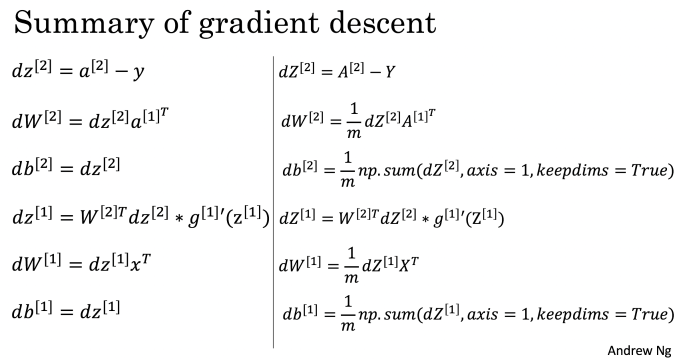
Implement the function backward_propagation().

Instructions: Backpropagation is usually the hardest (most mathematical) part in deep learning. The following figure is taken from is the slide from the lecture on backpropagation. We’ll want to use the six equations on the right of this slide, since we are building a vectorized implementation.

def backward_propagation(parameters, cache, X, Y):
    """
    Implement the backward propagation using the instructions above.
    
    Arguments:
    parameters -- python dictionary containing our parameters 
    cache -- a dictionary containing "Z1", "A1", "Z2" and "A2".
    X -- input data of shape (2, number of examples)
    Y -- "true" labels vector of shape (1, number of examples)
    
    Returns:
    grads -- python dictionary containing the gradients with respect to different parameters
    """

Implement the update rule. Use gradient descent. We have to use (dW1, db1, dW2, db2) in order to update (W1, b1, W2, b2).

General gradient descent rule: θ=θ−α(∂J/∂θ) where α is the learning rate and θ
represents a parameter.

Illustration: The gradient descent algorithm with a good learning rate (converging) and a bad learning rate (diverging). Images courtesy of Adam Harley.

def update_parameters(parameters, grads, learning_rate = 1.2):
    """
    Updates parameters using the gradient descent update rule given above
    
    Arguments:
    parameters -- python dictionary containing our parameters 
    grads -- python dictionary containing our gradients 
    
    Returns:
    parameters -- python dictionary containing our updated parameters 
    """

Integrate previous parts in nn_model()

Build the neural network model in nn_model().

Instructions: The neural network model has to use the previous functions in the right order.

def nn_model(X, Y, n_h, num_iterations = 10000, print_cost=False):
    """
    Arguments:
    X -- dataset of shape (2, number of examples)
    Y -- labels of shape (1, number of examples)
    n_h -- size of the hidden layer
    num_iterations -- Number of iterations in gradient descent loop
    print_cost -- if True, print the cost every 1000 iterations
    
    Returns:
    parameters -- parameters learnt by the model. They can then be used to predict.
    """

Predictions

Use the model to predict by building predict(). Use forward propagation to predict results.

def predict(parameters, X):
    """
    Using the learned parameters, predicts a class for each example in X
    
    Arguments:
    parameters -- python dictionary containing our parameters 
    X -- input data of size (n_x, m)
    
    Returns
    predictions -- vector of predictions of our model (red: 0 / blue: 1)
    """

It is time to run the model and see how it performs on a planar dataset. Run the following code to test our model with a single hidden layer of nh hidden units.

# Build a model with a n_h-dimensional hidden layer
parameters = nn_model(X, Y, n_h = 4, num_iterations = 10000, print_cost=True)

# Plot the decision boundary
plot_decision_boundary(lambda x: predict(parameters, x.T), X, Y)
plt.title("Decision Boundary for hidden layer size " + str(4))

Cost after iteration 0: 0.693048
Cost after iteration 1000: 0.288083
Cost after iteration 2000: 0.254385
Cost after iteration 3000: 0.233864
Cost after iteration 4000: 0.226792
Cost after iteration 5000: 0.222644
Cost after iteration 6000: 0.219731
Cost after iteration 7000: 0.217504
Cost after iteration 8000: 0.219471
Cost after iteration 9000: 0.218612

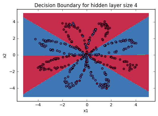
Cost after iteration 9000

0.218607

# Print accuracy
predictions = predict(parameters, X)
print ('Accuracy: %d' % float((np.dot(Y,predictions.T) + np.dot(1-Y,1-predictions.T))/float(Y.size)*100) + '%')

 Accuracy: 90%

Accuracy is really high compared to Logistic Regression. The model has learnt the leaf patterns of the flower! Neural networks are able to learn even highly non-linear decision boundaries, unlike logistic regression.

Now, let’s try out several hidden layer sizes. We can observe different behaviors of the model for various hidden layer sizes. The results are shown below.

Tuning hidden layer size

Accuracy for 1 hidden units: 67.5 %
Accuracy for 2 hidden units: 67.25 %
Accuracy for 3 hidden units: 90.75 %
Accuracy for 4 hidden units: 90.5 %
Accuracy for 5 hidden units: 91.25 %
Accuracy for 20 hidden units: 90.0 %
Accuracy for 50 hidden units: 90.25 %

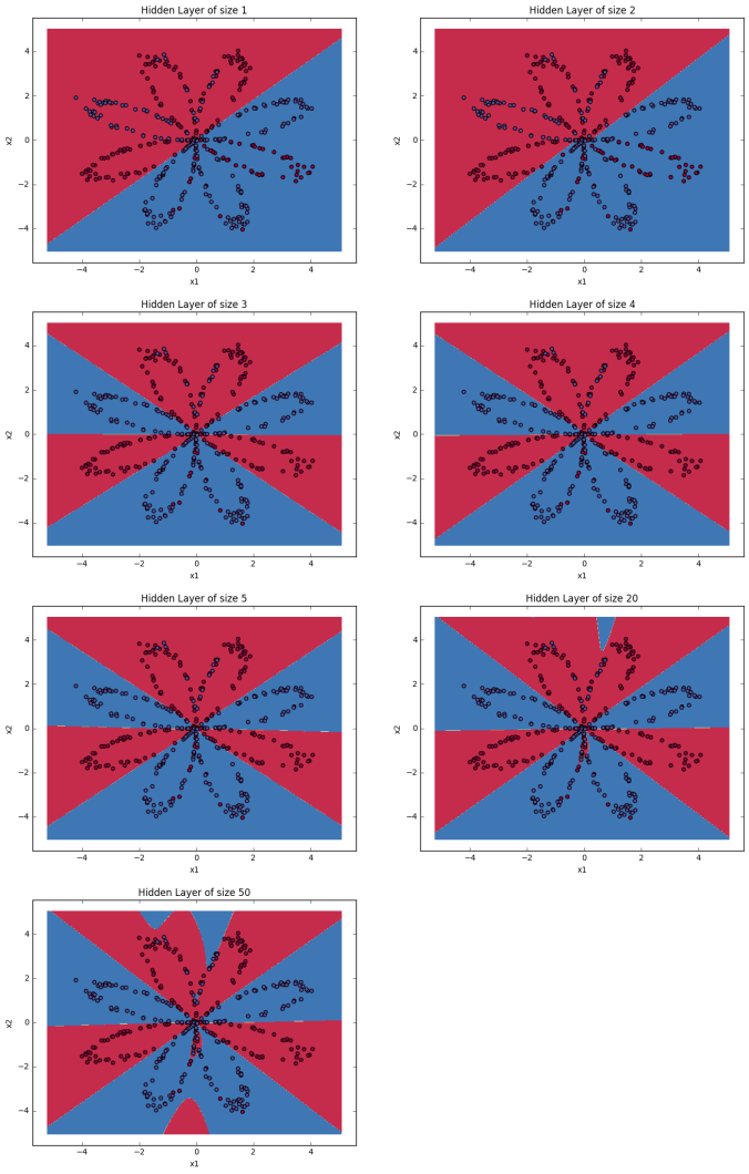
Interpretation:

• The larger models (with more hidden units) are able to fit the training set better, until eventually the largest models overfit the data.
• The best hidden layer size seems to be around n_h = 5. Indeed, a value around here seems to fits the data well without also incurring noticable overfitting.
• We shall also learn later about regularization, which lets us use very large models (such as n_h = 50) without much overfitting.

 

3. Getting deeper with Keras

 

• Tensorflow is a powerful and flexible tool, but coding large neural architectures with it is tedious.
• There are plenty of deep learning toolkits that work on top of it like Slim, TFLearn, Sonnet, Keras.
• Choice is matter of taste and particular task
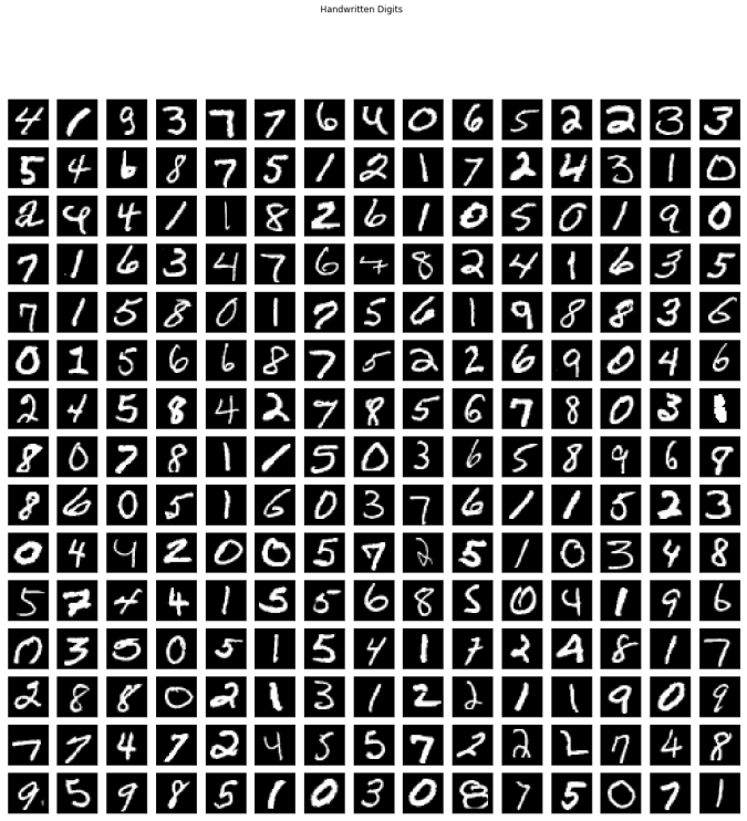
• We’ll be using Keras to predict handwritten digits with the mnist dataset.
• The following figure shows 225 sample images from the dataset.

 

 

The pretty keras

Using only the following few lines of code we can learn a simple deep neural net with 3 dense hidden layers and with Relu activation, with dropout 0.5 after each dense layer.

import keras
from keras.models import Sequential
import keras.layers as ll

model = Sequential(name="mlp")
model.add(ll.InputLayer([28, 28]))
model.add(ll.Flatten())

# network body
model.add(ll.Dense(128))
model.add(ll.Activation('relu'))
model.add(ll.Dropout(0.5))

model.add(ll.Dense(128))
model.add(ll.Activation('relu'))
model.add(ll.Dropout(0.5))

model.add(ll.Dense(128))
model.add(ll.Activation('relu'))
model.add(ll.Dropout(0.5))

# output layer: 10 neurons for each class with softmax
model.add(ll.Dense(10, activation='softmax'))

# categorical_crossentropy is our good old crossentropy
# but applied for one-hot-encoded vectors
model.compile("adam", "categorical_crossentropy", metrics=["accuracy"])

The following shows the summary of the model:

_________________________________________________________________
Layer (type)                 Output Shape              Param #   
=================================================================
input_12 (InputLayer)        (None, 28, 28)            0         
_________________________________________________________________
flatten_12 (Flatten)         (None, 784)               0         
_________________________________________________________________
dense_35 (Dense)             (None, 128)               100480    
_________________________________________________________________
activation_25 (Activation)   (None, 128)               0         
_________________________________________________________________
dropout_22 (Dropout)         (None, 128)               0         
_________________________________________________________________
dense_36 (Dense)             (None, 128)               16512     
_________________________________________________________________
activation_26 (Activation)   (None, 128)               0         
_________________________________________________________________
dropout_23 (Dropout)         (None, 128)               0         
_________________________________________________________________
dense_37 (Dense)             (None, 128)               16512     
_________________________________________________________________
activation_27 (Activation)   (None, 128)               0         
_________________________________________________________________
dropout_24 (Dropout)         (None, 128)               0         
_________________________________________________________________
dense_38 (Dense)             (None, 10)                1290      
=================================================================
Total params: 134,794
Trainable params: 134,794
Non-trainable params: 0
_________________________________________________________________

Model interface

Keras models follow Scikit-learn‘s interface of fit/predict with some notable extensions. Let’s take a tour.

# fit(X,y) ships with a neat automatic logging.
#          Highly customizable under the hood.
model.fit(X_train, y_train,
          validation_data=(X_val, y_val), epochs=13);

 Train on 50000 samples, validate on 10000 samples

Epoch 1/13
50000/50000 [==============================] - 14s - loss: 0.1489 - acc: 0.9587 - val_loss: 0.0950 - val_acc: 0.9758
Epoch 2/13
50000/50000 [==============================] - 12s - loss: 0.1543 - acc: 0.9566 - val_loss: 0.0957 - val_acc: 0.9735
Epoch 3/13
50000/50000 [==============================] - 11s - loss: 0.1509 - acc: 0.9586 - val_loss: 0.0985 - val_acc: 0.9752
Epoch 4/13
50000/50000 [==============================] - 11s - loss: 0.1515 - acc: 0.9577 - val_loss: 0.0967 - val_acc: 0.9752
Epoch 5/13
50000/50000 [==============================] - 11s - loss: 0.1471 - acc: 0.9596 - val_loss: 0.1008 - val_acc: 0.9737
Epoch 6/13
50000/50000 [==============================] - 11s - loss: 0.1488 - acc: 0.9598 - val_loss: 0.0989 - val_acc: 0.9749
Epoch 7/13
50000/50000 [==============================] - 11s - loss: 0.1495 - acc: 0.9592 - val_loss: 0.1011 - val_acc: 0.9748
Epoch 8/13
50000/50000 [==============================] - 11s - loss: 0.1434 - acc: 0.9604 - val_loss: 0.1005 - val_acc: 0.9761
Epoch 9/13
50000/50000 [==============================] - 11s - loss: 0.1514 - acc: 0.9590 - val_loss: 0.0951 - val_acc: 0.9759
Epoch 10/13
50000/50000 [==============================] - 11s - loss: 0.1424 - acc: 0.9613 - val_loss: 0.0995 - val_acc: 0.9739
Epoch 11/13
50000/50000 [==============================] - 11s - loss: 0.1408 - acc: 0.9625 - val_loss: 0.0977 - val_acc: 0.9751
Epoch 12/13
50000/50000 [==============================] - 11s - loss: 0.1413 - acc: 0.9601 - val_loss: 0.0938 - val_acc: 0.9753
Epoch 13/13
50000/50000 [==============================] - 11s - loss: 0.1430 - acc: 0.9619 - val_loss: 0.0981 - val_acc: 0.9761

As we could see, with a simple model without any convolution layers we could obtain more than 97.5% accuracy on the validation dataset.

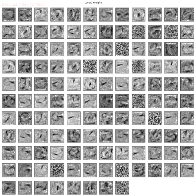
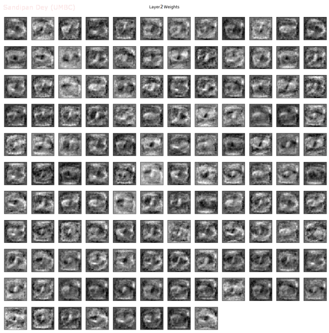
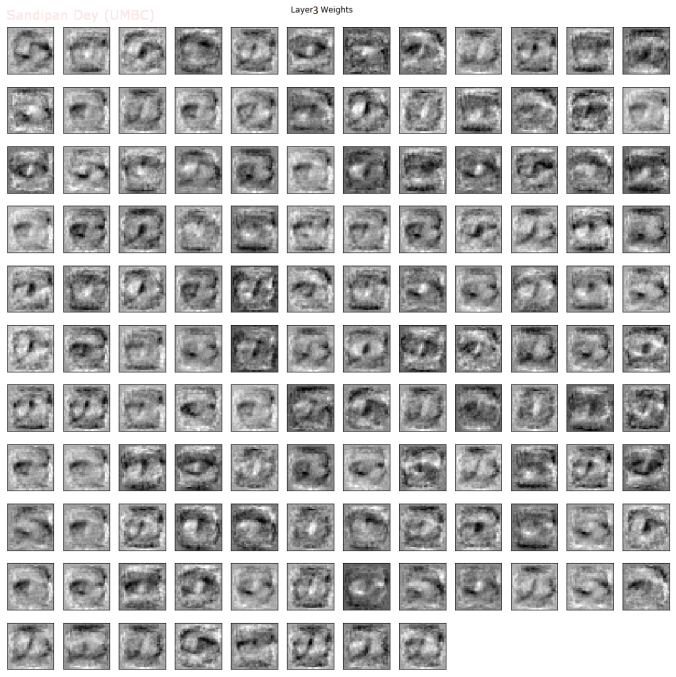
The following figures show the weights learnt at different layers.

Some Tips & tricks to improve accuracy

Here are some tips on what we can do to improve accuracy:

• Network size
  • More neurons,
  • More layers, (docs)
  • Nonlinearities in the hidden layers
    • tanh, relu, leaky relu, etc
  • Larger networks may take more epochs to train, so don’t discard the net just because it could didn’t beat the baseline in 5 epochs.

• Early Stopping
  • Training for 100 epochs regardless of anything is probably a bad idea.
  • Some networks converge over 5 epochs, others – over 500.
  • Way to go: stop when validation score is 10 iterations past maximum

• Faster optimization
  • rmsprop, nesterov_momentum, adam, adagrad and so on.
    • Converge faster and sometimes reach better optima
    • It might make sense to tweak learning rate/momentum, other learning parameters, batch size and number of epochs

• Regularize to prevent overfitting
  • Add some L2 weight norm to the loss function, theano will do the rest
    • Can be done manually or via – https://keras.io/regularizers/

• Data augmemntation – getting 5x as large dataset for free is a great deal
  • https://keras.io/preprocessing/image/
  • Zoom-in+slice = move
  • Rotate+zoom(to remove black stripes)
  • any other perturbations
  • Simple way to do that (if we have PIL/Image):
    • from scipy.misc import imrotate,imresize
    • and a few slicing
  • Stay realistic. There’s usually no point in flipping dogs upside down as that is not the way we usually see them.