Implementing Lucas-Kanade Optical Flow algorithm in Python

In this article an implementation of the Lucas-Kanade optical flow algorithm is going to be described. This problem appeared as an assignment in this computer vision course from UCSD. The inputs will be sequences of images (subsequent frames from a video) and the algorithm will output an optical flow field (u, v) and trace the motion of the moving objects. The problem description is taken from the assignment itself.

 

---

Problem Statement

---

---

Single-Scale Optical Flow

• Let’s implement the single-scale Lucas-Kanade optical flow algorithm. This involves finding the motion (u, v) that minimizes the sum-squared error of the brightness constancy equations for each pixel in a window.  The algorithm will be implemented as a function with the following inputs:

     def optical_flow(I1, I2, window_size, tau) # returns (u, v)

• Here, u and v are the x and y components of the optical flow, I1 and I2 are two images taken at times t = 1 and t = 2 respectively, and window_size is a 1 × 2 vector storing the width and height of the window used during flow computation.
• In addition to these inputs, a theshold τ should be added, such that if τ is larger than the smallest eigenvalue of A’A, then the the optical flow at that position should not be computed. Recall that the optical flow is only valid in regions where

has rank 2, which is what the threshold is checking. A typical value for τ is 0.01.

• We should try experimenting with different window sizes and find out the tradeoffs associated with using a small vs. a large window size.
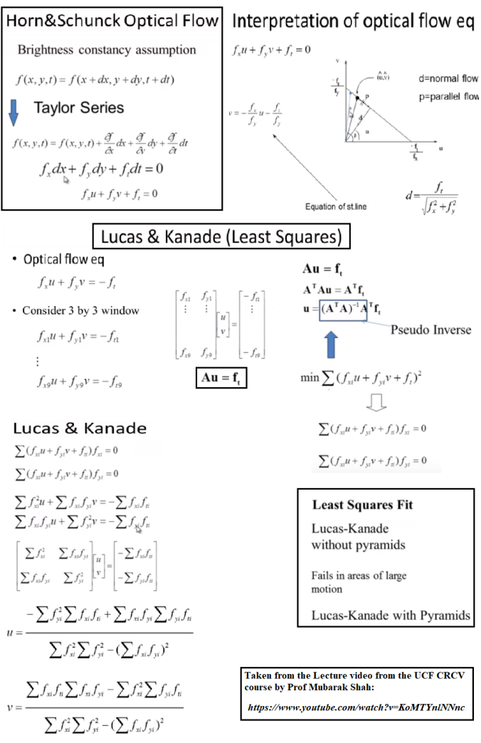
• The following figure describes the algorithm, which considers a nxn (n>=3) window around each pixel and solves a least-square problem to find the best flow vectors for the pixel.

• The following code-snippet shows how the algorithm is implemented in python for a gray-level image.

import numpy as np
from scipy import signal
def optical_flow(I1g, I2g, window_size, tau=1e-2):

    kernel_x = np.array([[-1., 1.], [-1., 1.]])
    kernel_y = np.array([[-1., -1.], [1., 1.]])
    kernel_t = np.array([[1., 1.], [1., 1.]])#*.25
    w = window_size/2 # window_size is odd, all the pixels with offset in between [-w, w] are inside the window
    I1g = I1g / 255. # normalize pixels
    I2g = I2g / 255. # normalize pixels
    # Implement Lucas Kanade
    # for each point, calculate I_x, I_y, I_t
    mode = 'same'
    fx = signal.convolve2d(I1g, kernel_x, boundary='symm', mode=mode)
    fy = signal.convolve2d(I1g, kernel_y, boundary='symm', mode=mode)
    ft = signal.convolve2d(I2g, kernel_t, boundary='symm', mode=mode) +
         signal.convolve2d(I1g, -kernel_t, boundary='symm', mode=mode)
    u = np.zeros(I1g.shape)
    v = np.zeros(I1g.shape)
    # within window window_size * window_size
    for i in range(w, I1g.shape[0]-w):
        for j in range(w, I1g.shape[1]-w):
            Ix = fx[i-w:i+w+1, j-w:j+w+1].flatten()
            Iy = fy[i-w:i+w+1, j-w:j+w+1].flatten()
            It = ft[i-w:i+w+1, j-w:j+w+1].flatten()
            #b = ... # get b here
            #A = ... # get A here
            # if threshold τ is larger than the smallest eigenvalue of A'A:
            nu = ... # get velocity here
            u[i,j]=nu[0]
            v[i,j]=nu[1]

    return (u,v)

 

---

Some Results

---

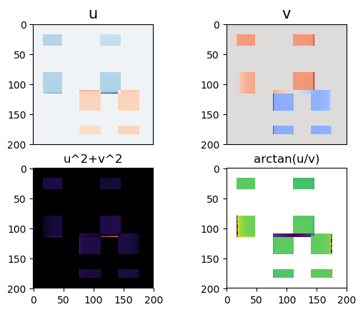
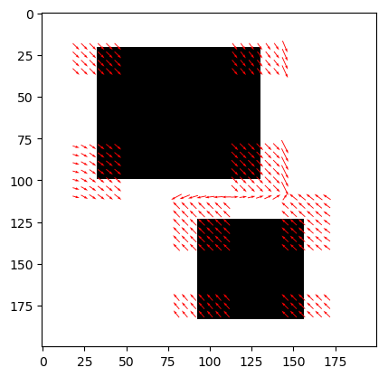
• The following figures and animations show the results of the algorithm on a few image sequences. Some of these input image sequences / videos are from the course and some are collected from the internet.
• As can be seen, the algorithm performs best if the motion of the moving object(s) in between consecutive frames is slow. To the contrary, if the motion is large, the algorithm fails and we should implement / use multiple-scale version Lucas-Kanade with image pyramids.
• Finally,  with small window size,  the algorithm captures subtle motions but not large motions. With large size it happens the other way.

---

---

Input Sequences

Output Optical Flow with different window sizes

window size = 15

window size = 21

 

---

---

Input Sequences

Output Optical Flow

---

---

Input Sequences (hamburg taxi)

Output Optical Flow

 

---

Input Sequences

Output Optical Flow

---

Input Sequences

Output Optical Flow

---

Input Sequences    

Output Optical Flow

---

Input Sequences

Output Optical Flow

---

Input Sequences

Output Optical Flow

---

Input Sequences
Output Optical Flow

---

Input Sequences

Output Optical Flow

Output Optical Flow

---

---

Input Sequences

Output Optical Flow with window size 45

Output Optical Flow with window size 10

Output Optical Flow with window size 25

Output Optical Flow with window size 45

---