Some more Social Network Analysis with Python: Centrality, PageRank/HITS, Random Network Generation Models, Link Prediction

In this article, some more social networking concepts will be illustrated with a few problems. The problems appeared in the programming assignments in the
coursera course Applied Social Network Analysis in Python.  The descriptions of the problems are taken from the assignments. The analysis is done using NetworkX.

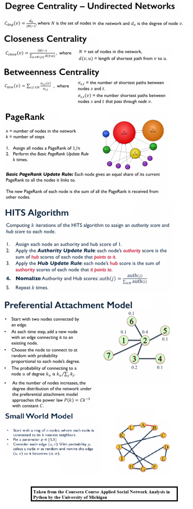
The following theory is going to be used to solve the assignment problems.

 

1. Measures of  Centrality

In this assignment, we explore measures of centrality on the following two networks:

1. A friendship network
2. A political blog network.

 

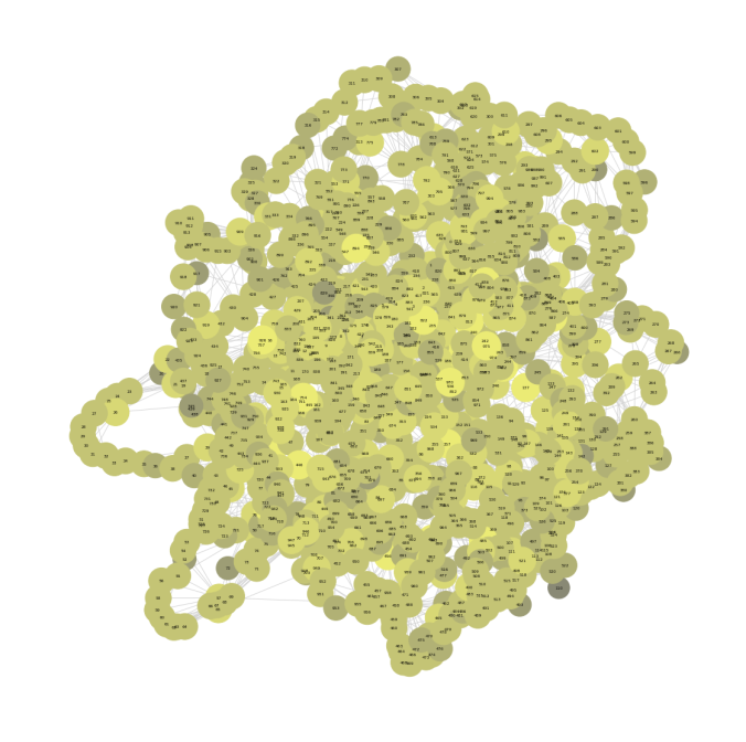
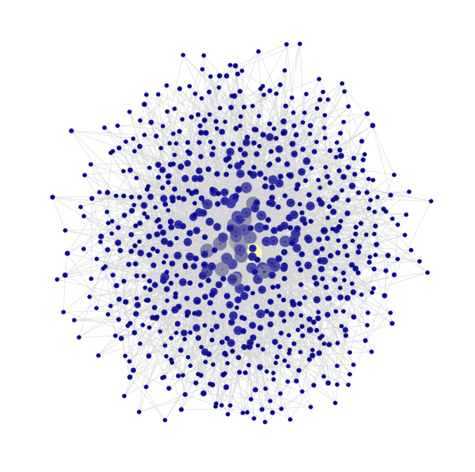
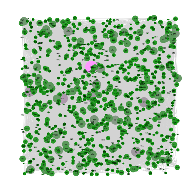
• First let’s do some analysis with different centrality measures using the friendship network, which is a network of friendships at a university department. Each node corresponds to a person, and an edge indicates friendship. The following figure visualizes the network, with the size of the nodes proportional to the degree of the nodes.

 

Degree Centrality

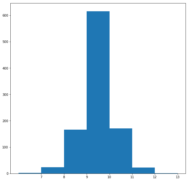
The next figure shows the distribution of the degree centrality of the nodes in the friendship network graph.

The following figure visualizes the network, with the size of the nodes again
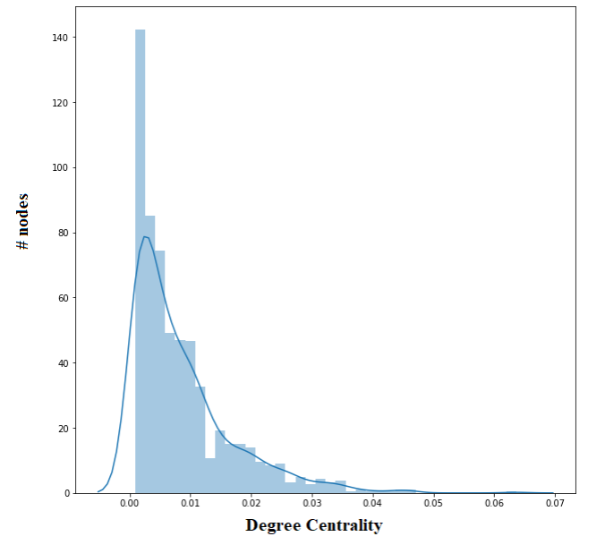
proportional to the degree centrality of the nodes.

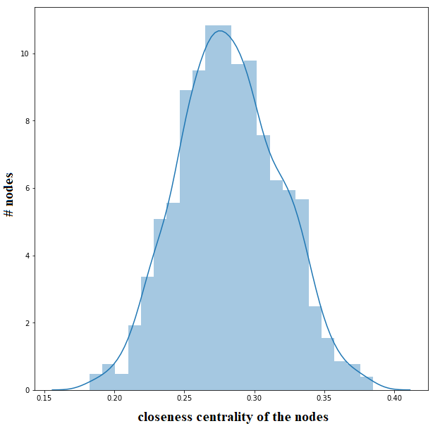
Closeness Centrality

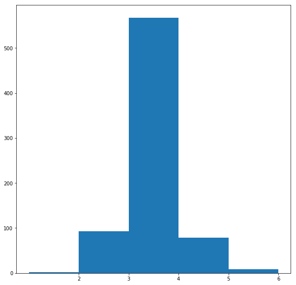
The next figure shows the distribution of the closeness centrality of the nodes in the friendship network graph.

 

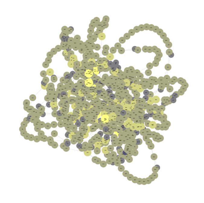
The following figure again visualizes the network, with the size of the nodes being
proportional to the closeness centrality of the nodes.

 

 

Betweenness Centrality

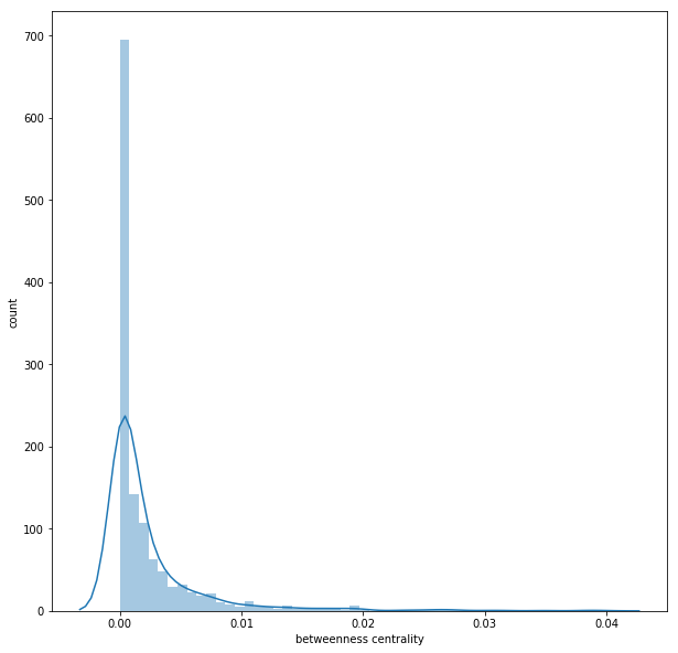
The next figure shows the distribution of the betweenness centrality of the nodes in the friendship network graph.

 

 

The following figure again visualizes the network, with the size of the nodes being
proportional to the betweenness centrality of the nodes.

 

 

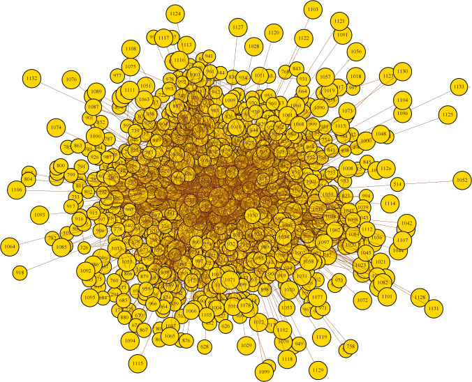
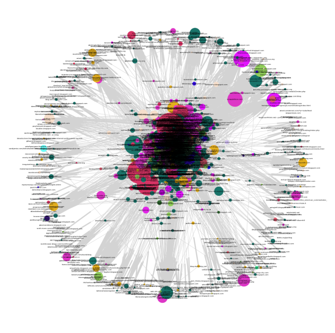
• Now, let’s consider another network, which is a directed network of political blogs, where nodes correspond to a blog and edges correspond to links between blogs.

• This network will be used to compute  the following:
  • PageRank of the nodes using random walk with damping factor.
  • Authority and Hub Score of the nodes using the HITS.

• The blog network looks like the following:
  

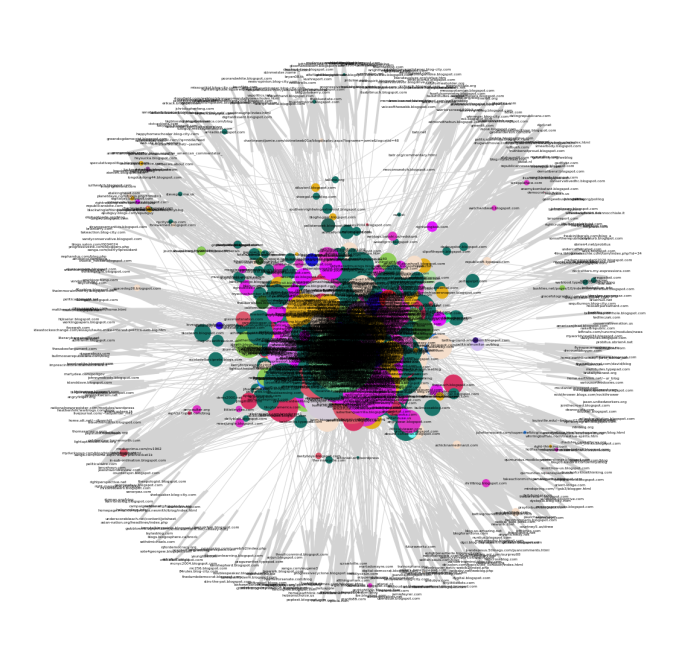
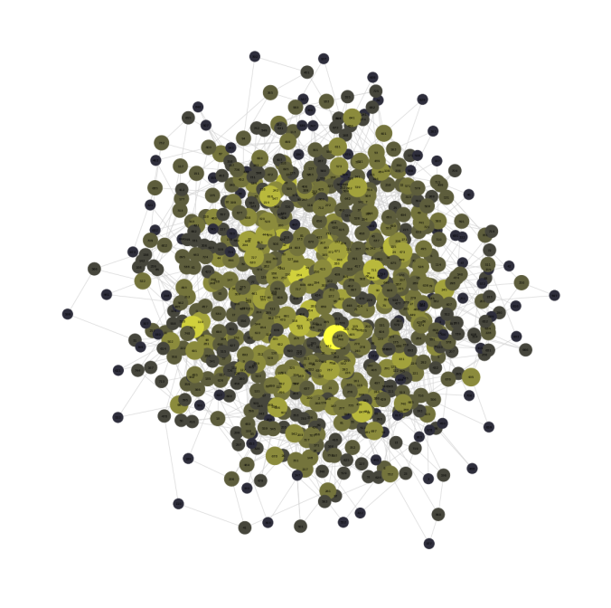
  	source	value
  tsrightdominion.blogspot.com	Blogarama	1
  rightrainbow.com	Blogarama	1
  gregpalast.com	LabeledManually	0
  younglibs.com	Blogarama	0
  blotts.org/polilog	Blogarama	0
  marylandpolitics.blogspot.com	BlogCatalog	1
  blogitics.com	eTalkingHead	0
  thesakeofargument.com	Blogarama	1
  joebrent.blogspot.com	Blogarama	0
  thesiliconmind.blogspot.com	Blogarama	0
  40ozblog.blogspot.com	Blogarama,BlogCatalog	0
  progressivetrail.org/blog.shtml	Blogarama	0
  randomjottings.net	eTalkingHead	1
  sonsoftherepublic.com	Blogarama	1
  rightvoices.com	CampaignLine	1
  84rules.blog-city.com	eTalkingHead	1
  blogs.salon.com/0002874	LeftyDirectory	0
  alvintostig.typepad.com	eTalkingHead	0
  notgeniuses.com	CampaignLine	0
  democratreport.blogspot.com	BlogCatalog	0

• First let’s visualize the network, next figure shows the visualization. The network has nodes (blogs) from 47 different unique sources, each node belonging to a source is colored with a unique color. The gray lines denote the edges (links) between the nodes (blogs).

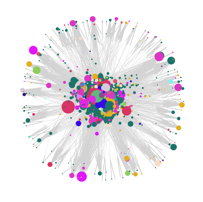
• The next figure shows the same network graph, but without the node labels (blog urls).

Page-Rank and HITS

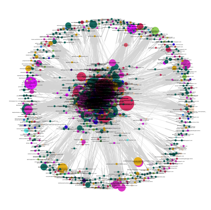
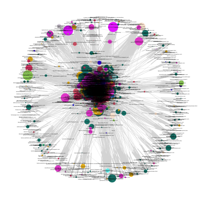
• Now, let’s apply the Scaled Page Rank Algorithm to this network.,with damping value 0.85. The following figure visualizes the graph with the node size proportional to the page rank of the node.
• The next animations show how the page rank of the nodes in the network changes with the first 25 iterations of the power-iteration algorithm.

 

• The top 5 nodes with the highest page rank values after 25 iterations of the power-iteration page-rank algorithm are shown below, along with their ranks scores.
  • (u’dailykos.com’, 0.020416972184975967)
  • (u’atrios.blogspot.com’, 0.019232277371918939)
  • (u’instapundit.com’, 0.015715941717833914)
  • (u’talkingpointsmemo.com’, 0.0152621016868163)
  • (u’washingtonmonthly.com’, 0.013848910355057181)

 

• The top 10 nodes with the highest page rank values after the convergence of the  page-rank algorithm are shown below, along with their ranks scores.
  • (u’dailykos.com’, 0.01790144388519838)
  • (u’atrios.blogspot.com’, 0.015178631721614688)
  • (u’instapundit.com’, 0.01262709066072975)
  • (u’blogsforbush.com’, 0.012508582138399093)
  • (u’talkingpointsmemo.com’, 0.012393033204751035)
  • (u’michellemalkin.com’, 0.010918873519905312)
  • (u’drudgereport.com’, 0.010712415519898428)
  • (u’washingtonmonthly.com’, 0.010512012551452737)
  • (u’powerlineblog.com’, 0.008939228332543162)
  • (u’andrewsullivan.com’, 0.00860773822610682)

 

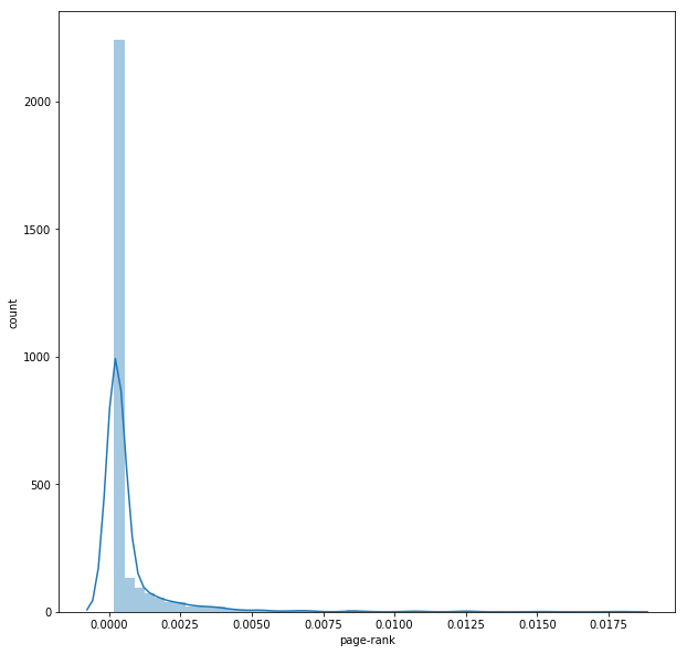
• The following figure shows the distribution of the page-ranks of the nodes after the convergence of the algorithm.

 

• Next, let’s apply the HITS Algorithm to the network to find the hub and authority scores of node.

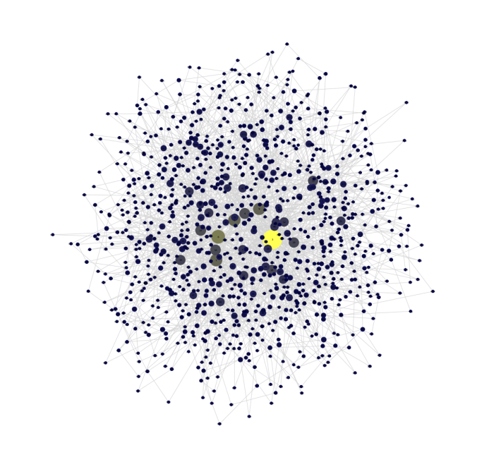
• The following couple of figures visualizes the network graph where the node size is proportional to the hub score and the authority score for the node respectively, once the HITS algorithm converges.
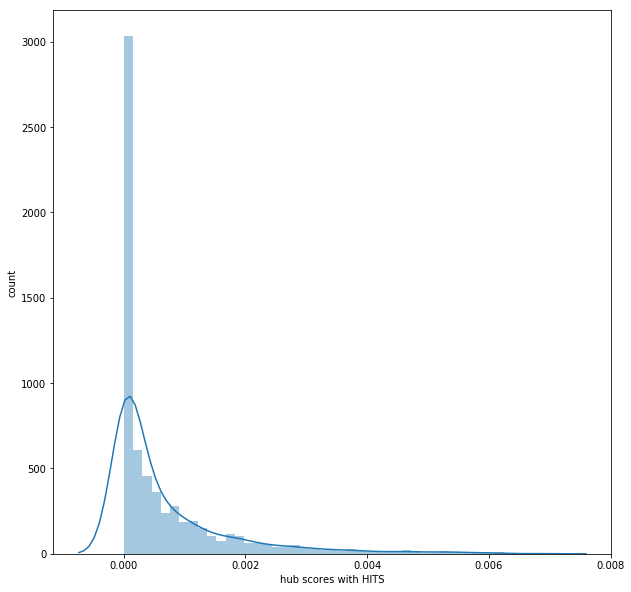
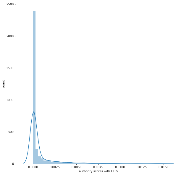
• Next couple of figures show the distribution of the hub-scores and the authority-scores for the nodes once the HITS converges.

 

• 

 

 

2. Random Graph Identification

 

Given a list containing 5 networkx graphs., with each of these graphs being generated by one of three possible algorithms:

• Preferential Attachment ('PA')
• Small World with low probability of rewiring ('SW_L')
• Small World with high probability of rewiring ('SW_H')

Anaylze each of the 5 graphs and determine which of the three algorithms generated the graph.

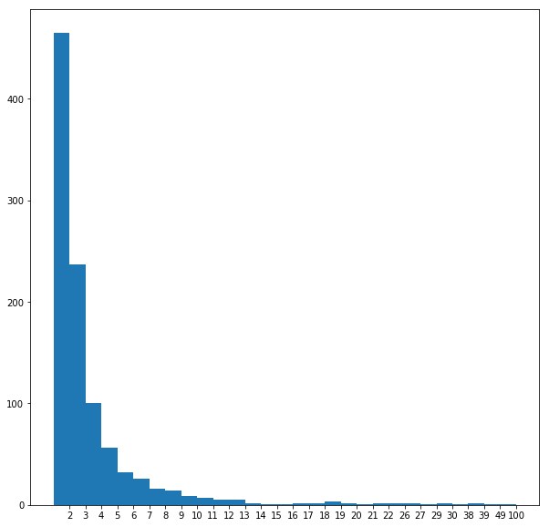
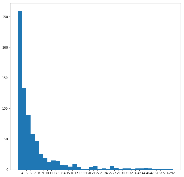
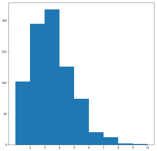
The following figures visualize all the graphs along with their degree-distributions. Since the Preferential Attachment model generates graphs with the node degrees following  the power-law distribution (since rich gets richer), the graphs with this pattern in their degree distributions are most likely generated by this model.

On the other hand, the Small World model generates graphs with the node degrees not following the power-law distribution, instead the distribution shows fat tails. If this pattern is seen, we can identify the network as to be generated with this model.

 

3. Prediction using Machine Learning models with the graph-centrality and local clustering features

 

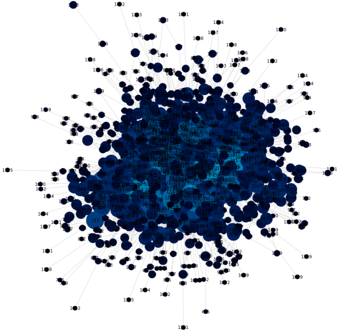
For this assignment we need to work with a company’s email network where each node corresponds to a person at the company, and each edge indicates that at least one email has been sent between two people.

The network also contains the node attributes Department and ManagmentSalary.

Department indicates the department in the company which the person belongs to, and ManagmentSalary indicates whether that person is receiving a managment position salary. The email-network graph has

• Number of nodes: 1005
• Number of edges: 16706
• Average degree: 33.2458

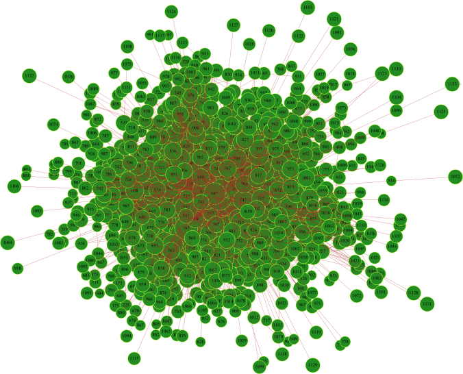
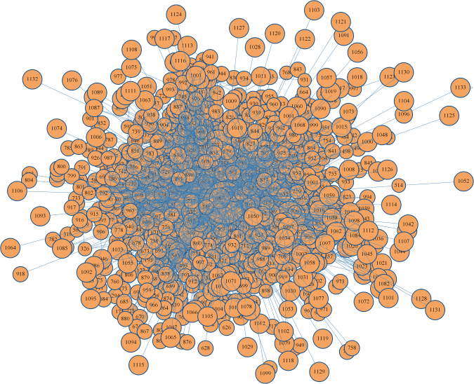
The following figure visualizes the email network graph.

Salary Prediction

Using network G, identify the people in the network with missing values for the node attribute ManagementSalary and predict whether or not these individuals are receiving a managment position salary.

To accomplish this, we shall need to

• Create a matrix of node features
• Train a (sklearn) classifier on nodes that have ManagementSalary data and
• Predict a probability of the node receiving a managment salary for nodes where ManagementSalary is missing.

The predictions will need to be given as the probability that the corresponding employee is receiving a managment position salary.

The evaluation metric for this assignment is the Area Under the ROC Curve (AUC).

A model needs to achieve an AUC of 0.75 on the test dataset.

Using the trained classifier, return a series with the data being the probability of receiving managment salary, and the index being the node id (from the test dataset).

The next table shows first few rows of the dataset with the degree and clustering features computed. The dataset contains a few ManagementSalary values are missing (NAN), the corresponding tuples form the test dataset, for which we need to predict the missing ManagementSalary values. The rest will be the training dataset.

Now,  a few classifiers will be trained on the training dataset , they are:

• RandomForest
• SVM
• GradientBoosting

with 3 input features for each node:

• Department
• Clustering (local clustering coefficient for the node)
• Degree

in order to predict the output variable as the indicator receiving  managment salary.

 

Index	Department	ManagementSalary	clustering	degree
0	1	0.0	0.276423	44
1	1	NaN	0.265306	52
2	21	NaN	0.297803	95
3	21	1.0	0.384910	71
4	21	1.0	0.318691	96
5	25	NaN	0.107002	171
6	25	1.0	0.155183	115
7	14	0.0	0.287785	72
8	14	NaN	0.447059	37
9	14	0.0	0.425320	40

 

Typical 70-30 validation is used for model selection. The next 3 tables show the first few rows of the train, validation and the test datasets respectively.

 

	Department	clustering	degree	ManagementSalary
421	14	0.227755	52	0
972	15	0.000000	2	0
322	17	0.578462	28	0
431	37	0.426877	25	0
506	14	0.282514	63	0
634	21	0.000000	3	0
130	0	0.342857	37	0
140	17	0.394062	41	0
338	13	0.350820	63	0
117	6	0.274510	20	0
114	10	0.279137	142	1
869	7	0.733333	6	0
593	5	0.368177	42	0
925	10	0.794118	19	1
566	14	0.450216	22	0
572	4	0.391304	26	0
16	34	0.284709	74	0
58	21	0.294256	126	1
57	21	0.415385	67	1
207	4	0.505291	30	0

 

Index	Department	clustering	degree	ManagementSalary
952	15	0.533333	8	0
859	32	0.388106	74	1
490	6	0.451220	43	0
98	16	0.525692	25	0
273	17	0.502463	31	0
784	28	0.000000	3	0
750	20	0.000000	1	0
328	8	0.432749	21	0
411	28	0.208364	106	1
908	5	0.566154	28	0
679	29	0.424837	20	0
905	1	0.821429	10	0
453	6	0.427419	34	1
956	14	0.485714	15	0
816	13	0.476190	23	0
127	6	0.341270	28	0
699	14	0.452899	26	0
711	21	0.000000	2	0
123	13	0.365419	36	0
243	19	0.334118	53	0

	Department	clustering	degree
1	1	0.265306	52
2	21	0.297803	95
5	25	0.107002	171
8	14	0.447059	37
14	4	0.215784	80
18	1	0.301188	56
27	11	0.368852	63
30	11	0.402797	68
31	11	0.412234	50
34	11	0.637931	31

The following table shows the first few predicted probabilities  by  the RandomForest classifier on the test dataset.

Index	0	1
0	1.0	0.0
1	0.2	0.8
2	0.0	1.0
3	1.0	0.0
4	0.5	0.5
5	1.0	0.0
6	0.7	0.3
7	0.7	0.3
8	0.3	0.7
9	0.7	0.3
10	0.9	0.1
11	0.8	0.2
12	1.0	0.0
13	0.6	0.4
14	0.7	0.3
15	0.5	0.5
16	0.0	1.0
17	0.2	0.8
18	1.0	0.0
19	1.0	0.0

 

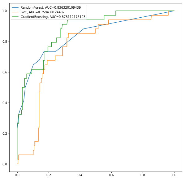
The next figure shows the ROC curve to compare the performances (AUC) of the classifiers on the validation dataset.

As can be seen, the GradientBoosting  classifier performs the best (has the highest AUC on the validation dataset).

 

 

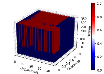
The following figure shows the Decision Surface for the Salary Prediction learnt by the RandomForest Classifier.

 

4. New Connections Prediction (Link Prediction with ML models)

For the last part of this assignment, we shall predict future connections between employees of the network. The future connections information has been loaded into the variable future_connections. The index is a tuple indicating a pair of nodes that currently do not have a connection, and the FutureConnectioncolumn indicates if an edge between those two nodes will exist in the future, where a value of 1.0 indicates a future connection. The next table shows first few rows of the dataset.

Index	Future Connection
(6, 840)	0.0
(4, 197)	0.0
(620, 979)	0.0
(519, 872)	0.0
(382, 423)	0.0
(97, 226)	1.0
(349, 905)	0.0
(429, 860)	0.0
(309, 989)	0.0
(468, 880)	0.0

 

Using network G and future_connections, identify the edges  in future_connections
with missing values and predict whether or not these edges will have a future connection.

To accomplish this, we shall need to

1. Create a matrix of features for the edges found in future_connections
2. Train a (sklearn) classifier on those edges in future_connections that have Future Connection data
3. Predict a probability of the edge being a future connection for those edges in future_connections where Future Connection is missing.

The predictions will need to be given as the probability of the corresponding edge being a future connection.

The evaluation metric for this assignment is again the Area Under the ROC Curve (AUC).

Using the trained classifier, return a series with the data being the probability of the edge being a future connection, and the index being the edge as represented by a tuple of nodes.

Now,  a couple of classifiers will be trained on the training dataset , they are:

• RandomForest
• GradientBoosting

with 2 input features for each edge:

• Preferential attachment
• Common Neighbors

in order to predict the output variable Future Connection.

The next table shows first few rows of the dataset with the preferential attachment and Common Neighbors  features computed.

Index	Future Connection	preferential attachment	Common Neighbors
(6, 840)	0.0	2070	9
(4, 197)	0.0	3552	2
(620, 979)	0.0	28	0
(519, 872)	0.0	299	2
(382, 423)	0.0	205	0
(97, 226)	1.0	1575	4
(349, 905)	0.0	240	0
(429, 860)	0.0	816	0
(309, 989)	0.0	184	0
(468, 880)	0.0	672	1
(228, 715)	0.0	110	0
(397, 488)	0.0	418	0
(253, 570)	0.0	882	0
(435, 791)	0.0	96	1
(711, 737)	0.0	6	0
(263, 884)	0.0	192	0
(342, 473)	1.0	8140	12
(523, 941)	0.0	19	0
(157, 189)	0.0	6004	5
(542, 757)	0.0	90	0

 

Again, typical 70-30 validation is used for model selection. The next 3 tables show the first few rows of the train, validation and the test datasets respectively.

 

	preferential attachment	Common Neighbors	Future Connection
(7, 793)	360	0	0
(171, 311)	1620	1	0
(548, 651)	684	2	0
(364, 988)	18	0	0
(217, 981)	648	0	0
(73, 398)	124	0	0
(284, 837)	132	1	0
(748, 771)	272	4	0
(79, 838)	88	0	0
(207, 716)	90	1	1
(270, 928)	15	0	0
(201, 762)	57	0	0
(593, 620)	168	1	0
(494, 533)	18212	40	1
(70, 995)	18	0	0
(867, 997)	12	0	0
(437, 752)	205	0	0
(442, 650)	28	0	0
(341, 900)	351	0	0
(471, 684)	28	0	0

 

Index	preferential attachment	Common Neighbors	Future Connection
(225, 382)	150	0	0
(219, 444)	594	0	0
(911, 999)	3	0	0
(363, 668)	57	0	0
(161, 612)	2408	4	0
(98, 519)	575	0	0
(59, 623)	636	0	0
(373, 408)	2576	6	0
(948, 981)	27	0	0
(690, 759)	44	0	0
(54, 618)	765	0	0
(149, 865)	330	0	0
(562, 1001)	320	1	1
(84, 195)	4884	10	1
(421, 766)	260	0	0
(599, 632)	70	0	0
(814, 893)	10	0	0
(386, 704)	24	0	0
(294, 709)	75	0	0
(164, 840)	864	3	0

 

	preferential attachment	Common Neighbors
(107, 348)	884	2
(542, 751)	126	0
(20, 426)	4440	10
(50, 989)	68	0
(942, 986)	6	0
(324, 857)	76	0
(13, 710)	3600	6
(19, 271)	5040	6
(319, 878)	48	0
(659, 707)	120	0

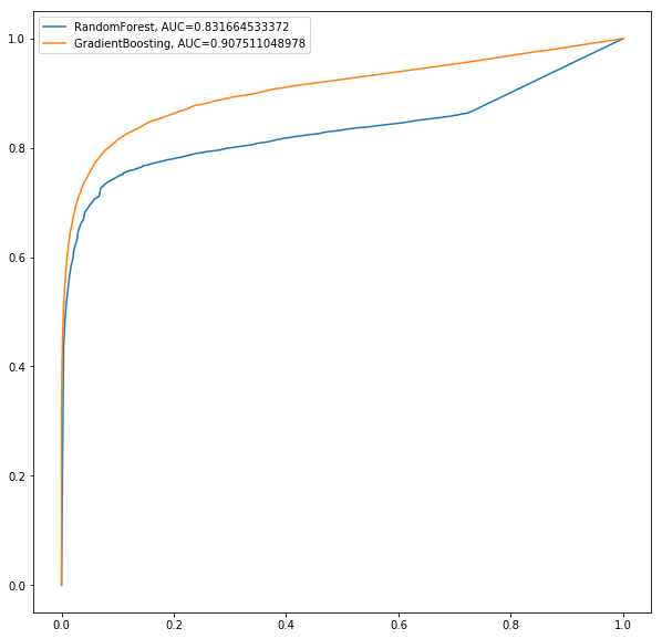
The next figure shows the ROC curve to compare the performances (AUC) of the classifiers on the validation dataset.

As can be seen, the GradientBoosting  classifier again performs the best (has the highest AUC on the validation dataset).

 

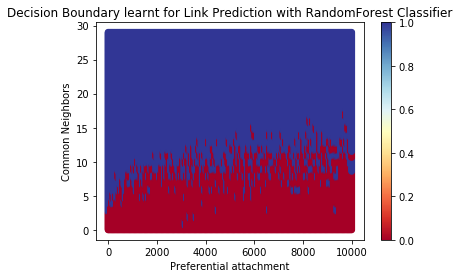
The following figure shows the Decision Boundary for the Link Prediction learnt by the RandomForest Classifier.